Projects
Near and Far
OSIRIS-REx: Image Analysis at NASA
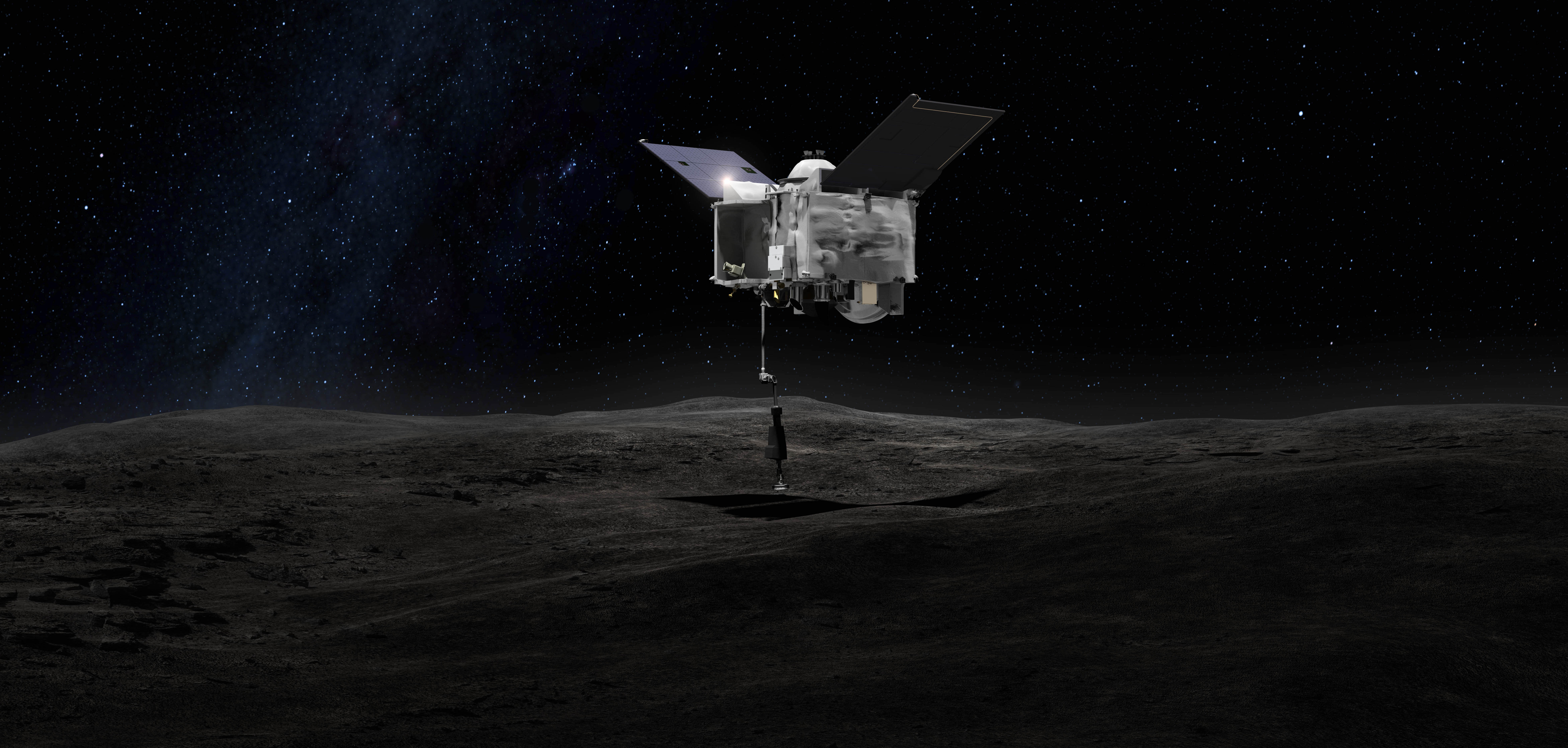
In the summer of 2018, I worked with NASA Goddard Space Flight Center on OSIRIS-REx, a spacecraft bound for the asteroid Bennu, where it would collect a small sample and return it to Earth in September 2023.
We chose Bennu for a few reasons:
- It's close. Bennu's orbit lies between Earth and Mars, which is a viable distance to fly to and launch a return capsule from.
- It is old. This bad boy is as old as the Solar System, so it can provide valuable insight into how planetary systems formed, including our very own.
- It has ingredients for the origin of life. Our telescopes tell us that Bennu is rich in carbon and organic compounds. Voyaging to Bennu allows us to study the role of asteroids as a way of bringing life to Earth.
- It can wipe out humanity! Bennu could potentially hit Earth in ~250 years, although the chances are super low (about 1 in 2,700). Still, it'd be nice to scope out a potential threat to humanity's existence, you know?
Analyzing Mid-Flight Images
As an intern at NASA Goddard, I was tasked with analyzing mid-flight images beamed back from OSIRIS-REx, which at this point had been rocketing towards Bennu for 18 months of its 27-month journey. Essentially, I was checking to make sure nothing wonky was going wrong with the cameras after 1.5 years in space.
In more technical language, I was to construct the 2D point spread functions (PSFs) of some target stars that the cameras imaged at certain regions in the camera's field-of-view (FOV). Do you know what a point spread function is? I certainly didn't! Going into the project, I knew nothing about PSFs, image cross-correlation, or anything related to optics except for some small section in my lower-division physics courses.
Fortunately, this man, my fabulous mentor Dr. Brent Bos, changed that.

What is a PSF?
Imagine you're taking a photo of a star. In optics, we make the simplification that because the star is so far away, it appears as a point source. Of course, with physics rearing its ugly head, this ideal point source concept gets destroyed by
- Lens aberrations
- Finite pixel size (can't represent a point source perfectly if your pixels aren't infinitesimally small themselves!)
- Quantum mechanical effects, like diffraction
Technical note: the PSF is the impulse response of an optical system, or the output you get when you feed in an impulse, which in our 2D case is a point source. The image you actually see is the convolution of the true image with the PSF. If you know your PSF, you can use it in a deconvolution algorithm (popular: Richardson-Lucy) to estimate the true image. This is important if you want a good pic of your space rock!
PSF Data from OSIRIS-REx
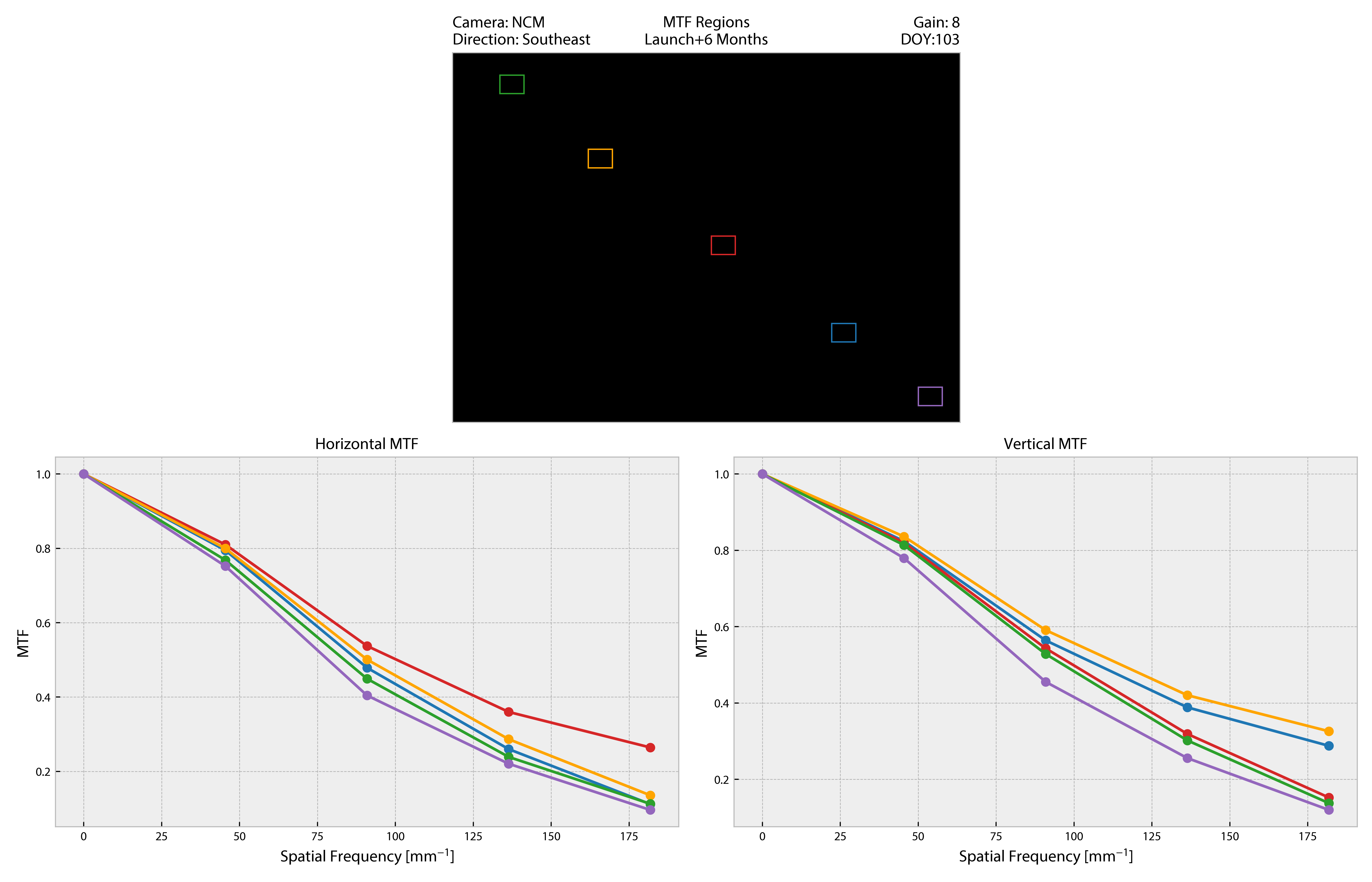
For this project, we analyzed the PSFs from images in data captured at 6 months (L+6) and at 18 months (L+18) after OSIRIS-REx launched. The goal was to examine the change in camera quality over time. At L+6 and L+18, OSIRIS-REx imaged the stars Fomalhaut and Pollux, respectively, at different regions of the camera to test the system response over the camera's FOV.
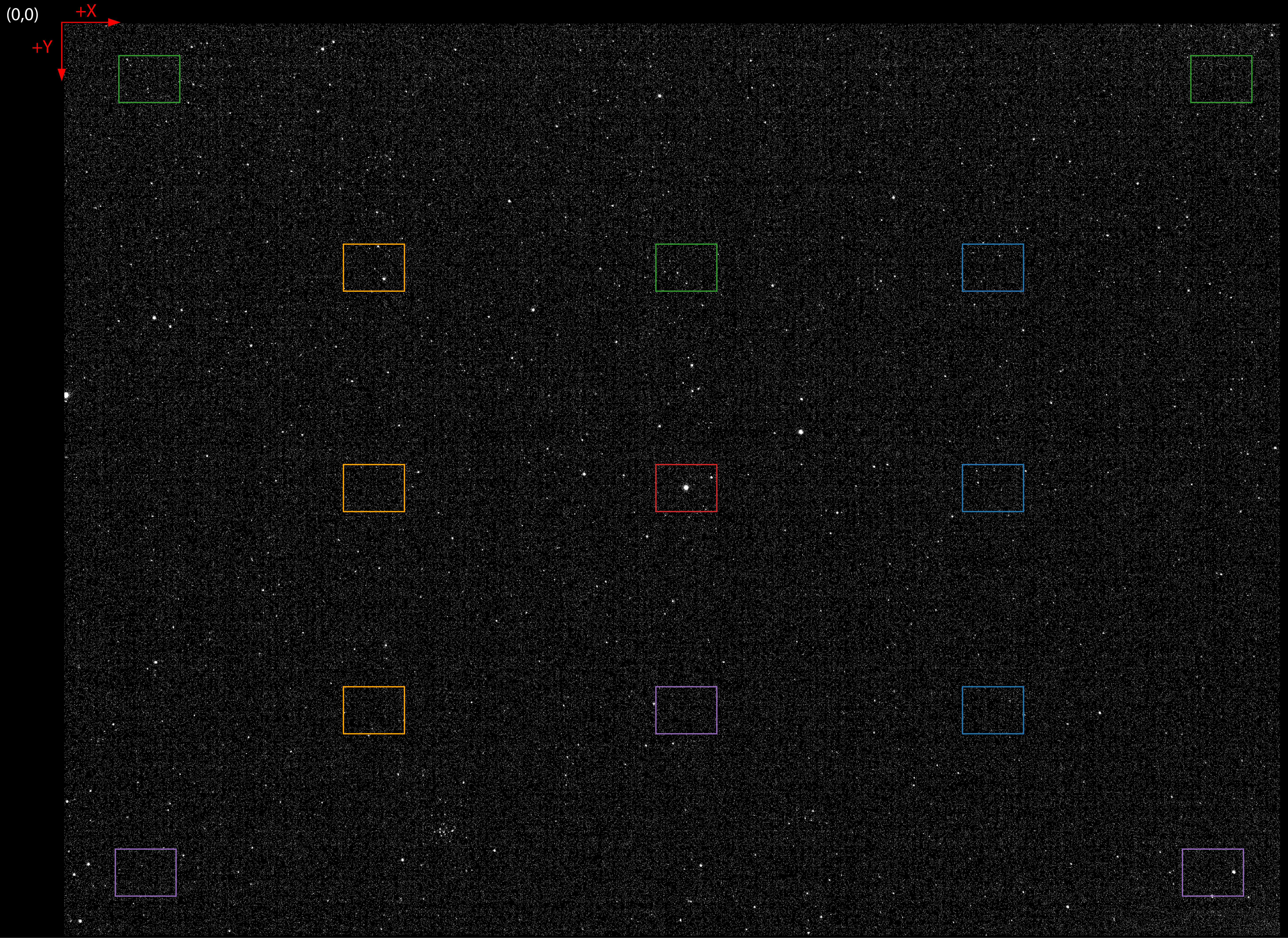
Here's a display showing all calibration locations in the FOV, with the target in the center for this specific image.
Before we inspect the PSFs, we need to preprocess these images. Always preprocess your images.
Dark Frame Subtraction
First, to improve the signal-to-noise ratio (SNR) and get a better image of the calibration star, we performed some dark frame subtraction, which is considered standard for space-based image sensors.
All image sensors are suspectible to noise. At longer exposures, the noise in these sensors has more time to accumulate, making your object of interest harder to see. Fortunately, the fix is quite simple: take a picture (or several averaged together) with the lens cap over the camera, giving you the mean noise—noise we can simply subtract off from a real image. We call this the "dark frame."
I had it even easier, since all this calibration was done before my arrival to Goddard! Since we had a known dark frame, I just subtracted it from every image to remove the average noise. Plain and simple.
Combining PSFs
Before we continue our quest for higher signal-to-noise, I must add that during the calibration campaign at L+6 months and L+18 months, the team took images of Pollux/Fomalhaut with a 0.5s exposure time and with a 5s exposure time in the same locations. We observed the following:
- The 0.5s exposure PSFs contained good data at the centers, but weren't bright enough at the edges.
- The 5s exposure PSF centers were oversaturated, but they contained valuable PSF information at the edges.
- When switching exposures from 0.5s to 5s, there was a non-negligible pointing error star, such that the 0.5s and 5s PSF images didn't line up.
The team deliberately planned the first two points, but the third was unexpected. Brent and I devised a method to fuse the information from the two exposures into one PSF, what we called "hybrid PSFs."
In brief, to construct these hybrid PSFs, we
- Divide out the exposure time to normalize the 0.5s and 5s PSFs to the same scale.
- Use a cross-correlation to find the pixel shift between the 0.5s and 5s PSF images.
- Upsample the 0.5s PSFs, shift them to line up with the 5s PSFs, then downsample to their original size.
- Replace every saturated pixel (i, j) in the 5s image with its counterpart pixel (i, j) in the 0.5s image.
If you're interested, more details can be found in our paper.
Here are the constructed hybrid PSFs, positioned where they were captured in the FOV.
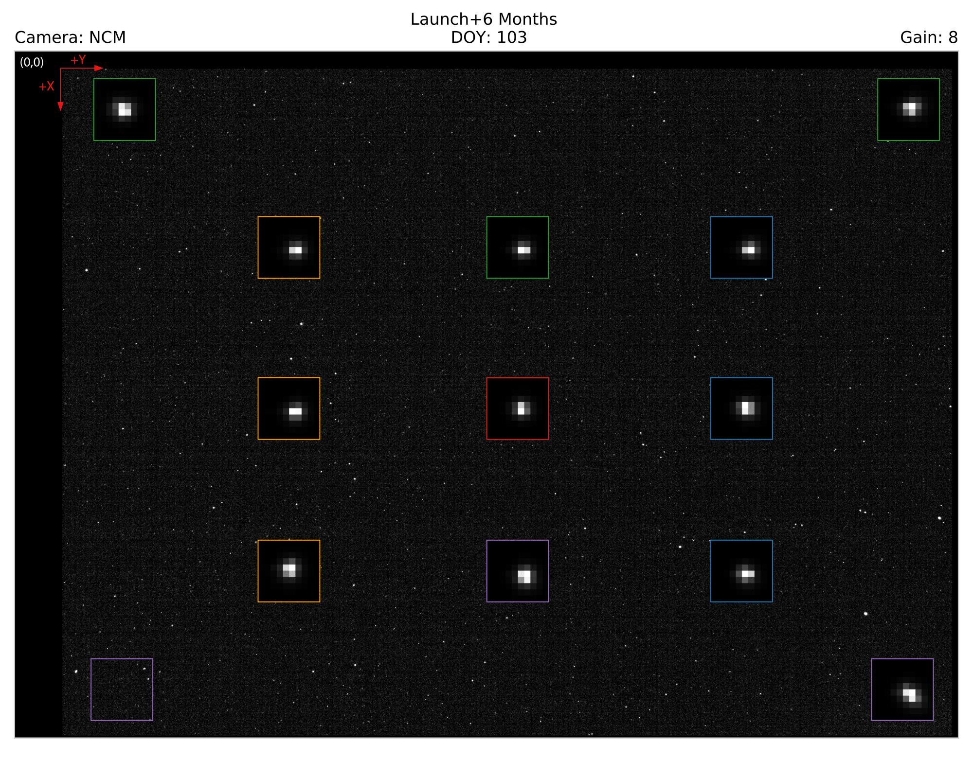
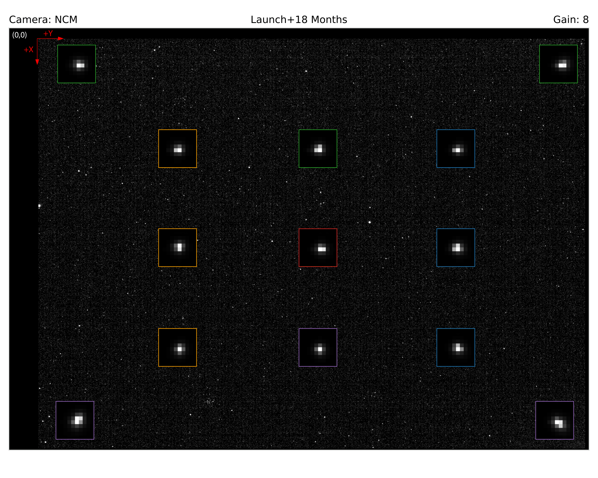
Right: Hybrid PSFs 18 months after launch.
When comparing the L+6 to L+18 month images, these PSFs don't look too different at first glance, which is good! Again, more "spread out" PSFs means more blurring of point sources which would mean a degradation in image quality. We don't see much change here, indicating that image quality remained stable over time.
Going Deeper: The Modulation Transfer Function
Unfortunately, we can't just look at two pictures, say they look similar, and call it a day. We actually have to look at numbers! Plots! Graphs! So, let's take a look at something called the MTF.
At a high level, the modulation transfer function (what a mouthful), or MTF, measures the ability to show contrast at a given level of detail. All optical systems start out being able to contrast larger image details very well, and the level of contrast drops as the system has to resolve tinier details. The MTF sets out to measure how well an optical system can preserve spatial details.
Technical note: the MTF is magnitude of the optical system's response as a function of the input's spatial frequencies. Smell like Fourier to you? It is! While the PSF measures the system's impulse response, we can get the complex-valued optical transfer function (OTF) by Fourier transforming the PSF. The MTF is simply the magnitude, or absolute value, of the OTF—the phase component gets dropped. In math lingo, we have
$$ OTF(\nu) = \mathfrak{F}\{PSF\} \\ MTF(\nu) = \| OTF(\nu) \| = \| \mathfrak{F}\{PSF\} \| $$
where $\mathfrak{F}$ denotes the Fourier transform.
Below are some MTFs at a diagonal sweep through the FOV for images taken at L+6 and L+18 months. The "horizontal MTF" originates from using only a horizontal profile of the PSF for the MTF; likewise for the "vertical MTF." I didn't know what I was doing back then.
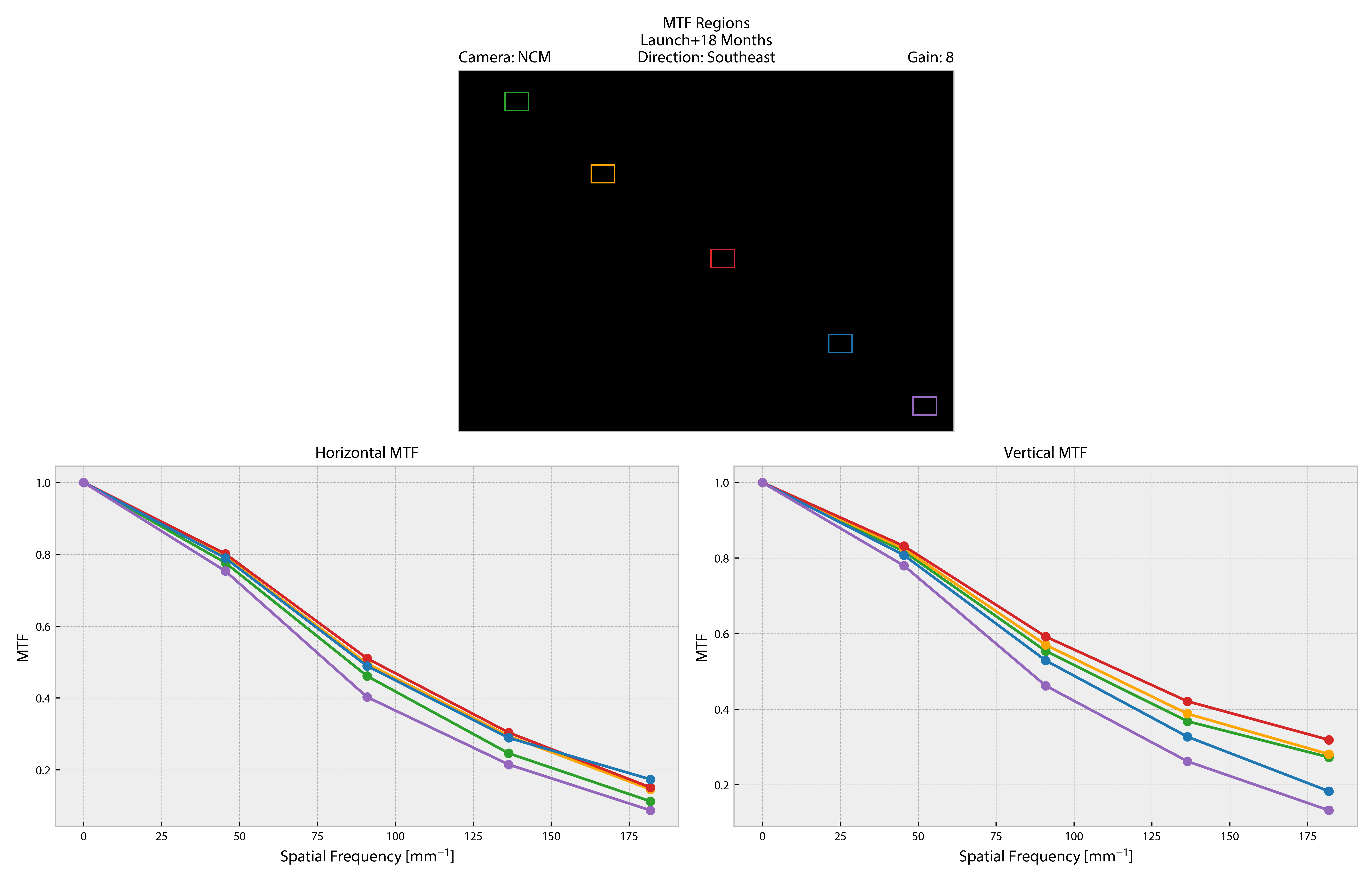
Bottom: NavCam 1 (NCM) MTFs for images taken 18 months after launch (L+18).
The MTF colors correspond to the region of the FOV where the target star was imaged.
Looking at the horizontal and vertical MTFs between the two calibration campaigns, we see that the MTFs don't vary significantly with time. Furthermore, these mid-flight results agree with pre-launch ground tests to within measurement noise, indicating no outstanding degradation of the cameras. Nice.
In short, our mid-flight analysis of the OSIRIS-REx cameras demonstrated that the cameras remained consistent 1.5 years into the spacecraft's journey towards Bennu. At the time of writing, OSIRIS-REx had successfully and dramatically captured a sample from the asteroid on October 20, 2020 and is now rocketing back to Earth, hopefully returning in September 2023.
Thanks, NASA friends!
I'm super fortunate to have this opportunity, especially since I didn't know anything as a sophomore in undergrad. Thanks to the NASA Goddard Optics Branch and Dr. Brent Bos for setting me up for a fantastic career. Be sure to read the paper if you're interested in the rest of the mid-flight camera calibration!
Paper: In-Flight Calibration and Performance of the OSIRIS-REx Touch And Go Camera System (TAGCAMS)